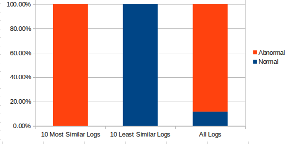
Logs are one of the first places I look when an embedded system behaves unexpectedly. They are also one of the worst places to work at scale. A single test run can produce more output than a person can read carefully, and months of nightly testing turn that into a search problem: which runs deserve an engineer's attention first?
For a CS 589 machine learning project, I explored whether Sentence Transformer embeddings could make that search tractable. The goal was not to replace an engineer or declare a root cause automatically. It was to build a local ranking system that could compare a new batch of logs with previous runs, push unusual files toward the top, and eventually point toward the lines contributing most to the difference.
The source data came from proprietary system testing, so privacy was a design constraint rather than an afterthought. The pipeline ran locally, and the figures in this post contain only aggregate labels and numerical results. No raw log messages, internal identifiers, hostnames, or product details are included.
Why Semantic Similarity?
The simplest anomaly detector for logs is a search for words such as "error" or "failed." That works for explicit failures, but it misses many of the cases that make debugging difficult: a sequence that ends early, an operation that takes an unusual amount of time, or a run whose messages are individually ordinary but collectively different from the baseline.
Sentence Transformers offered a way to compare meaning rather than exact strings. The core pipeline was:
- Read each log and split it into individual messages.
- Normalize high-variance fields, especially timestamps.
- Encode the cleaned text into dense vectors with a BERT-based Sentence Transformer.
- Compute pairwise cosine similarity between log embeddings.
- Average each row of the similarity matrix to give every log a rough similarity-to-the-group score.
- Sort those scores and inspect the most- and least-similar tails.
The matrix is useful because it preserves relationships that a single anomaly score hides. A low-scoring run might be an isolated failure, while a block of mutually similar runs can reveal a recurring failure mode. The ranking then turns that structure into something operational: start with the unusual tail instead of reading files in chronological order.
Preprocessing Was Part of the Model
My first experiments used minimal preprocessing. They looked promising because the encoder appeared to find strongly dissimilar runs. Closer inspection changed the story. Absolute timestamps varied everywhere, and that superficial difference could dominate the representation. After converting timestamps to relative offsets, several models produced similarity values extremely close to 1.0 across many files.
That was an important failure. The original variation was not necessarily evidence that the model understood system behavior; it was partly evidence that timestamps were different.
Relative time was still worth preserving. Removing time completely would throw away signals such as long pauses or unexpectedly compressed sequences. The better tradeoff was to normalize every run to a common starting point, retaining timing relationships without letting calendar time identify the file. Grouping logs by test type also made comparisons more meaningful: a run should be judged against runs that attempted the same kind of work.
Memory became another practical limit. Encoding whole collections of long logs with BERT-based models is expensive, so early experiments were capped at 100 smaller files. A production version would need batching, incremental embedding, and more aggressive removal of repetitive boilerplate.
Comparing Off-the-Shelf Encoders
I compared three popular Sentence Transformer families:
- all-MiniLM-L6-v2, a compact model designed for semantic search and clustering
- LaBSE, a multilingual model built to align meaning across languages
- msmarco-bert-base-dot-v5, a retrieval-oriented model trained around semantic search
all-MiniLM-L6-v2 was the most natural starting point. It is relatively small, fast, and explicitly useful for clustering. LaBSE tested whether a broader embedding space would help, while the msmarco model offered a retrieval-focused alternative.
None of them cleanly separated the domain out of the box. The least-similar tail from the untuned MiniLM model still mixed normal and abnormal runs:
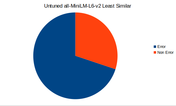
The other encoders showed the same larger problem: general semantic similarity is not the same as operational similarity. Two logs can discuss the same subsystem and still represent very different outcomes. Conversely, a successful run and a failed run can share most of their vocabulary. The models knew language, but they did not yet know what counted as abnormal in this system.
Teaching the Model the Domain
The next step was supervised fine-tuning. I divided the available runs into two labeled groups: abnormal logs that warranted investigation and normal logs that passed inspection. From those groups I created pairs:
- Two logs from the same group received a similarity target of
1. - A normal/abnormal pair received a similarity target of
0.
I fine-tuned all-MiniLM-L6-v2 using CosineSimilarityLoss. The initial setup used a batch size of 16, four epochs, and 100 warmup steps. Later experiments increased training to 10 epochs, extended warmup, and added weight decay. I also moved to data with a healthier balance between the two classes, because a detector trained mostly on failures can learn a distorted picture of normal behavior.
The useful lesson from hyperparameter tuning was not that one magic value solved the problem. Warmup, regularization, and additional epochs each changed the tail composition, but those changes had to be judged on held-out logs. A smoother training run means little if the anomaly queue is still mixed.
After domain-specific training, the separation became much clearer. In the reported tuned result, the ten least-similar files were all normal, while the ten most-similar files were all abnormal:
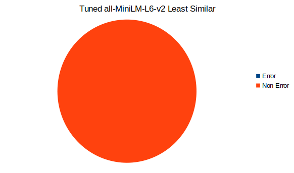
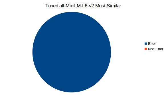
Those labels may look reversed at first. The score is similarity to the full collection, not a direct probability of failure. Because the dataset contained many more abnormal than normal runs, abnormal logs formed the dominant cluster and appeared in the most-similar tail. Normal logs were rarer, so they appeared less similar to the group overall. This is exactly why an anomaly score needs context: the minority class is not automatically the class an engineer cares about.
Evaluation: Ranking Before Classification
The project framed evaluation in terms of true positives and false negatives because missing an important run is more costly than reviewing an extra one. But the first practical diagnostic was tail composition: after sorting by average similarity, did one end contain a useful concentration of one class, or were both ends still mixed?
This is not a substitute for a complete confusion matrix. It is a test of whether the representation is useful enough to support triage. If the first ten files an engineer opens are all from the same meaningful group, the ranking has immediate value even before choosing a production threshold. The next evaluation step would set that threshold on a held-out set, report precision and recall for the abnormal class, and tune explicitly for a low false-negative rate.
Qualitative review matters too. A mathematically unusual log is only useful if an engineer agrees that it represents something worth investigating. The strongest version of this system would combine quantitative evaluation with feedback on whether the ranking shortened real debugging sessions.
What I Learned
Preprocessing can create or destroy the signal. The early timestamp-driven result looked encouraging until normalization exposed it. In log ML, fields that are valuable to a human can become shortcuts for a model.
General-purpose embeddings need domain supervision. The off-the-shelf encoders were good at broad semantic similarity but not at the operational distinction this task required. A relatively small amount of labeled pair training made the embedding space more relevant.
Class balance changes what "anomalous" means. Average similarity finds distance from the dominant group. If failures dominate the dataset, a normal run can look like the anomaly. Labels, sampling strategy, and the intended operational question have to agree.
Ranking is often a better first product than automatic classification. A ranked queue supports the engineer without pretending the model has perfect confidence. It also creates a natural feedback loop for collecting better labels.
Local-first architecture can be a feature. Sensitive logs do not need to leave the environment to benefit from transformer models. Keeping preprocessing, inference, and evaluation local narrowed the security surface and made it easier to reason about what could be published.
Where I Would Take It Next
The most valuable next feature is line-level attribution. Once a log is ranked as unusual, the system should compare its messages with the nearest baseline and highlight the lines that contribute most to the difference. That turns "this file is unusual" into a useful starting point for diagnosis.
I would also batch embeddings, cache unchanged files, evaluate chronologically to avoid leakage between related test runs, and calibrate a threshold against a held-out set. Finally, I would track performance by test type rather than relying on one global score; behavior that is normal for one scenario may be deeply unusual for another.
The project started as an attempt to search a mountain of text. It ended up teaching a broader lesson about applied machine learning: the hard part is rarely choosing the largest model. It is defining the comparison, removing shortcuts, building an evaluation that matches the real decision, and preserving the context that makes the result useful.