Long Short-Term Memory (LSTM) networks are particularly well-suited for time series prediction tasks. Unlike traditional feedforward networks, LSTMs can learn long-term dependencies in sequential data, making them ideal for forecasting stock prices, weather patterns, and other temporal phenomena.
Why LSTMs for Time Series?
Time series data has inherent temporal dependencies—future values depend on past values. LSTMs excel at:
- Capturing long-term patterns in sequential data
- Handling variable-length sequences
- Learning from context across many time steps
- Dealing with non-stationary data (trends, seasonality)
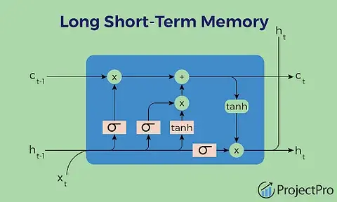
Understanding LSTM Architecture
LSTMs use a gated mechanism to control information flow:
- Forget Gate: Decides what information to discard
- Input Gate: Determines what new information to store
- Output Gate: Controls what information to output
This architecture allows LSTMs to maintain long-term memory while selectively updating it.
Building an LSTM Model with TensorFlow/Keras
Here's a complete example for stock price prediction:
import numpy as np
import pandas as pd
from tensorflow.keras.models import Sequential
from tensorflow.keras.layers import LSTM, Dense, Dropout, LayerNormalization
from tensorflow.keras.callbacks import EarlyStopping
from sklearn.preprocessing import MinMaxScaler

class PricePredictor:
    def __init__(self, sequence_length=60, n_features=1):
        self.sequence_length = sequence_length
        self.n_features = n_features
        self.scaler = MinMaxScaler()
        self.model = None

    def prepare_data(self, data, train_size=0.7, val_size=0.15):
        """Prepare time series data for LSTM training"""
        # Normalize data
        scaled_data = self.scaler.fit_transform(data.values.reshape(-1, 1))

        # Create sequences
        X, y = [], []
        for i in range(self.sequence_length, len(scaled_data)):
            X.append(scaled_data[i-self.sequence_length:i, 0])
            y.append(scaled_data[i, 0])

        X, y = np.array(X), np.array(y)
        X = X.reshape((X.shape[0], X.shape[1], self.n_features))

        # Split data
        train_end = int(len(X) * train_size)
        val_end = train_end + int(len(X) * val_size)

        X_train, y_train = X[:train_end], y[:train_end]
        X_val, y_val = X[train_end:val_end], y[train_end:val_end]
        X_test, y_test = X[val_end:], y[val_end:]

        return (X_train, y_train), (X_val, y_val), (X_test, y_test)

    def build_model(self, lstm_units=[128, 64, 32, 16], dropout_rate=0.2):
        """Build multi-layer LSTM model"""
        model = Sequential()

        # First LSTM layer with return_sequences=True
        model.add(LSTM(
            units=lstm_units[0],
            return_sequences=True,
            input_shape=(self.sequence_length, self.n_features)
        ))
        model.add(LayerNormalization())
        model.add(Dropout(dropout_rate))

        # Additional LSTM layers
        for units in lstm_units[1:-1]:
            model.add(LSTM(units=units, return_sequences=True))
            model.add(LayerNormalization())
            model.add(Dropout(dropout_rate))

        # Final LSTM layer
        model.add(LSTM(units=lstm_units[-1], return_sequences=False))
        model.add(LayerNormalization())
        model.add(Dropout(dropout_rate))

        # Output layer
        model.add(Dense(units=1))

        model.compile(
            optimizer='adam',
            loss='mse',
            metrics=['mae']
        )

        self.model = model
        return model

    def train(self, X_train, y_train, X_val, y_val, epochs=100, batch_size=32):
        """Train the model with early stopping"""
        early_stopping = EarlyStopping(
            monitor='val_loss',
            patience=10,
            restore_best_weights=True,
            verbose=1
        )

        history = self.model.fit(
            X_train, y_train,
            validation_data=(X_val, y_val),
            epochs=epochs,
            batch_size=batch_size,
            callbacks=[early_stopping],
            verbose=1
        )

        return history

    def predict(self, X):
        """Make predictions and inverse transform"""
        predictions = self.model.predict(X)
        return self.scaler.inverse_transform(predictions)
Key Design Decisions
Sequence Length
The sequence length determines how much historical data the model considers:
# Shorter sequences (30-60): Faster training, less context
# Longer sequences (100+): More context, slower training
sequence_length = 60  # Good balance for daily stock prices
Multi-Layer Architecture
Stacking LSTM layers allows the model to learn hierarchical patterns:
# Each layer learns different levels of abstraction
# First layer: Short-term patterns
# Deeper layers: Long-term trends and relationships
Dropout and Regularization
Prevent overfitting with dropout and layer normalization:
model.add(Dropout(0.2))  # 20% of neurons randomly disabled
model.add(LayerNormalization())  # Normalize activations
Training Strategies
Early Stopping
Monitor validation loss to prevent overfitting:
early_stopping = EarlyStopping(
    monitor='val_loss',
    patience=10,  # Stop after 10 epochs without improvement
    restore_best_weights=True
)
Learning Rate Scheduling
Adjust learning rate during training:
from tensorflow.keras.callbacks import ReduceLROnPlateau

lr_scheduler = ReduceLROnPlateau(
    monitor='val_loss',
    factor=0.5,
    patience=5,
    min_lr=1e-7
)
Evaluation Metrics
For time series prediction, use appropriate metrics:
from sklearn.metrics import mean_squared_error, mean_absolute_error

def evaluate_predictions(y_true, y_pred):
    mse = mean_squared_error(y_true, y_pred)
    mae = mean_absolute_error(y_true, y_pred)
    rmse = np.sqrt(mse)

    # Mean Absolute Percentage Error
    mape = np.mean(np.abs((y_true - y_pred) / y_true)) * 100

    return {
        'MSE': mse,
        'MAE': mae,
        'RMSE': rmse,
        'MAPE': f'{mape:.2f}%'
    }
Common Pitfalls and Solutions
1. Data Leakage
Problem: Using future data to predict past values
Solution: Ensure proper temporal splitting—never shuffle time series data randomly.
2. Overfitting
Problem: Model memorizes training data but fails on new data
Solution: Use dropout, early stopping, and sufficient validation data.
3. Non-Stationary Data
Problem: Trends and seasonality make predictions difficult
Solution: Consider differencing, detrending, or using more sophisticated architectures.
Real-World Application: Stock Price Prediction
In my LSTM Stock Price Prediction project, I implemented:
- Multi-layer architecture with 4 LSTM layers
- Dropout regularization (0.2) to prevent overfitting
- Layer normalization for stable training
- Early stopping to find optimal training duration
- Comprehensive evaluation with MSE, MAE, and visualizations
The model learns patterns in historical stock prices to predict future closing prices, though it's important to remember that stock markets are inherently unpredictable.
Conclusion
LSTM networks are powerful tools for time series prediction. Success requires careful architecture design, proper data preparation, and thoughtful evaluation. Start with simple models, iterate based on results, and gradually add complexity as needed.
Remember: time series prediction is challenging, and no model can perfectly predict the future. Focus on building robust systems that provide useful insights while acknowledging their limitations.